C30 Scalable Data Processing in R
Table of Contents
- 1. Working With Increasingly Large Data Sets
- 1.1. What is scalable data processing?
- 1.2. Why is your code slow?
- 1.3. How does processing time vary by data size?
- 1.4. Working with "Out-of-Core" Objects using the Bigmemory Project
- 1.5. Reading a big.matrix object
- 1.6. Attaching a big.matrix object
- 1.7. Creating tables with big.matrix objects
- 1.8. Data summary using
bigsummary - 1.9. References vs. Copies
- 1.10. Copying matrices and big matrices
- 2. Processing and Analyzing Data with
bigmemory- 2.1. The Bigmemory Suite of Packages
- 2.2. Tabulating using
bigtable - 2.3. Borrower Race and Ethnicity by Year (I)
- 2.4. Split-Apply-Combine
- 2.5. Female Proportion Borrowing
- 2.6. Split
- 2.7. Apply
- 2.8. Combine
- 2.9. Visualize your results using the tidyverse
- 2.10. Visualizing Female Proportion Borrowing
- 2.11. The Borrower Income Ratio
- 2.12. Tidy Big Tables
- 2.13. Limitations of bigmemory
- 2.14. Where should you use
bigmemory?
Important note: Given the IP statements, we can not publish the DataCamp videos of this course.
Datasets are often larger than available RAM, which causes problems for R programmers since by default all the variables are stored in memory. You’ll learn tools for processing, exploring, and analyzing data directly from disk. you’ll also implement the Split-Apply-Combine approach and learn how to write scalable code using the bigmemory and iotools packages. In this course, you'll make use of the Federal Housing Finance Agency's data, a publicly available data set chronicling all mortgages that were held or securitized by both Federal National Mortgage Association (Fannie Mae) and Federal Home Loan Mortgage Corporation (Freddie Mac) from 2009-2015.
1 Working With Increasingly Large Data Sets
In this chapter, we cover the reasons you need to apply new techniques when data sets are larger than available RAM. we show that importing and exporting data using the base R functions can be slow and some easy ways to remedy this. Finally, we introduce the bigmemory package.
1.1 What is Scalable Data Processing?
video
slides
1.2 Why is your code slow?
Reading and writing data to the hard drive takes much longer than reading and writing to RAM. This means if you need to retrieve data from the hard drive it takes much longer to move it to the CPU - where it can be processed - compared to moving data from RAM to the CPU. A program's use of resources, like RAM, processors, and hard drive dictate how quickly your R code runs. You can't change these resources without physically swapping them out for other hardware. However, you can often use the resources you have more efficiently. In particular, if you have a data set that is about the size of RAM, you might be better off saving most of the data set on the disk. By loading only the parts of a data set you need, you free up resources so that each part can be processed more quickly.
Which one of the following does not contribute to processing time?
Answer the question
Possible Answers
[ ]The complexity of your analysis.[ ]How much data you have to import from the hard drive.[ ]How fast your CPU is.[X]The time your code took to write.
How long it takes to write code and how long it takes to run code are independent.
1.3 How does processing time vary by data size?
If you are processing all elements of two data sets, and one data set is bigger, then the bigger data set will take longer to process. However, it's important to realize that how much longer it takes is not always directly proportional to how much bigger it is. That is, if you have two data sets and one is two times the size of the other, it is not guaranteed that the larger one will take twice as long to process. It could take 1.5 times longer or even four times longer. It depends on which operations are used to process the data set.
In this exercise, you'll use the microbenchmark package, which was
covered in the Writing Efficient R Code course.
Note: Numbers are specified using scientific notation
\(1e5 = 1 \times 10^{5} = 100000\)
1.3.1 Instructions
- Load the
microbenchmarkpackage. - Use the
microbenchmark()function to compare the sort times of random vectors. - Call
plot()on mb.
## Load the microbenchmark package
Install_And_Load <- function(Required_Packages)
{
        Remaining_Packages <- Required_Packages[!(Required_Packages %in%
                                                  installed.packages()[,"Package"])];

        if(length(Remaining_Packages))
        {
                install.packages(Remaining_Packages, repos='http://cran.rstudio.com/');
        }
        for(package_name in Required_Packages)
        {
                library(package_name,character.only=TRUE,quietly=TRUE);
        }
}

writeLines("\n :: Install new package: microbenchmark ...")
## Specify the list of required packages to be installed and load
Required_Packages <- c("microbenchmark")
## Call the Function
Install_And_Load(Required_Packages);
writeLines("\n :: Library microbenchmark loaded...")

## -------------------------------------------------------------------

## Compare the timings for sorting different sizes of vector
mb <- microbenchmark(
        ## Sort a random normal vector length 1e5
        "1e5" = sort(rnorm(1e5)),
        ## Sort a random normal vector length 2.5e5
        "2.5e5" = sort(rnorm(2.5e5)),
        ## Sort a random normal vector length 5e5
        "5e5" = sort(rnorm(5e5)),
        "7.5e5" = sort(rnorm(7.5e5)),
        "1e6" = sort(rnorm(1e6)),
        times = 10
)

## Plot the resulting benchmark object
## plot(mb)
:: Install new package: microbenchmark ...

:: Library microbenchmark loaded...
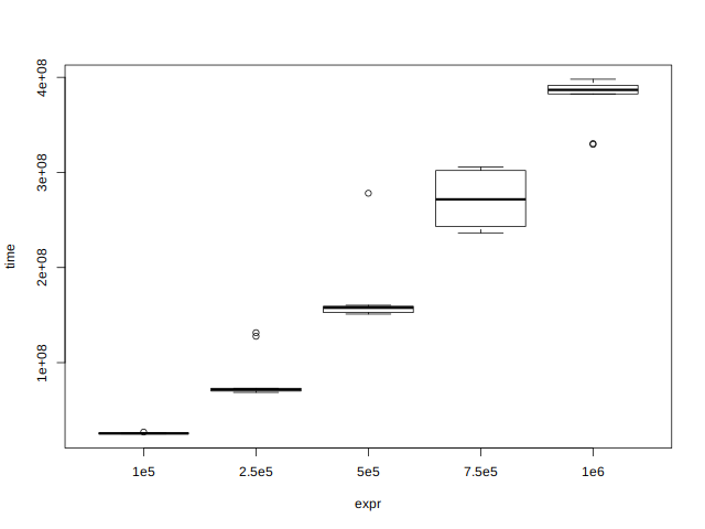
Figure 1: Comparing microbenchmark vectors
Note that the resulting graph shows that the execution time is not the same every time. This is because while the computer was executing your R code, it was also doing other things. As a result, it is a good practice to run each operation being benchmarked mutiple times, and to look at the median execution time when evaluating the execution time of R code.
1.4 Working with "Out-of-Core" Objects using the Bigmemory Project
video
1.5 Reading a big.matrix object
In this exercise, you'll create your first file-backed big.matrix
object using the read.big.matrix() function. The function is meant to
look similar to read.table() but, in addition, it needs to know what
type of numeric values you want to read ("char", "short", "integer",
"double"), it needs the name of the file that will hold the matrix's
data (the backing file), and it needs the name of the file to hold
information about the matrix (a descriptor file). The result will be a
file on the disk holding the value read in along with a descriptor
file which holds extra information (like the number of columns and
rows) about the resulting big.matrix object.
1.5.1 Instructions
- Load the
bigmemorypackage. - Use the
read.big.matrix()function to read a file called"mortgage-sample.csv", which contains a header and is composed of integer values. In addition:- Create a backingfile called
"mortgage-sample.bin", and - A descriptor file called
"mortgage-sample.desc".
- Create a backingfile called
- Find the dimensions of
xusing thedim()function.
## Load the bigmemory package
Install_And_Load <- function(Required_Packages)
{
        Remaining_Packages <- Required_Packages[!(Required_Packages %in%
                                                  installed.packages()[,"Package"])];

        if(length(Remaining_Packages))
        {
                install.packages(Remaining_Packages, repos='http://cran.rstudio.com/');
        }
        for(package_name in Required_Packages)
        {
                library(package_name,character.only=TRUE,quietly=TRUE);
        }
}

writeLines("\n :: Install new package: bigmemory ...")
## Specify the list of required packages to be installed and load
Required_Packages <- c("bigmemory")
## Call the Function
Install_And_Load(Required_Packages);
writeLines("\n :: Library bigmemory loaded...")
## -------------------------------------------------------------------
destfile <- "../data/mortgage-sample.csv"

if(!file.exists(destfile)) {
        download.file(url = "https://assets.datacamp.com/production/course_2399/datasets/mortgage-sample.csv",
                      destfile = destfile)
}

## Create the big.matrix object: x
x <- read.big.matrix(destfile, header = TRUE,
         type = "integer",
         backingfile = "mortgage-sample.bin",
         descriptorfile = "mortgage-sample.desc",
         backingpath = "../data")

## Find the dimensions of x
dim(x)
 :: Install new package: bigmemory ...

 :: Library bigmemory loaded...
[1] 70000    16
1.6 Attaching a big.matrix object
Now that the big.matrix object is on the disk, we can use the
information stored in the descriptor file to instantly make it
available during an R session. This means that you don't have to
reimport the data set, which takes more time for larger files. You can
simply point the bigmemory package at the existing structures on the
disk and begin accessing data without the wait.
1.6.1 Instructions
The big.matrix object x is available in your workspace.
- Create a new variable
mortthat points toxby attaching the"mortgage-sample.desc"file using theattach.big.matrix()function. - Verify that the dimensions of
mortare the same as the last exercise. - Call
head()onmort.
## Attach mortgage-sample.desc
mort <- attach.big.matrix("mortgage-sample.desc",
                          path = "../data")

## Find the dimensions of mort
dim(mort)

## Look at the first 6 rows of mort
head(mort)
[1] 70000    16
     enterprise record_number msa perc_minority tract_income_ratio
[1,]          1           566   1             1                  3
[2,]          1           116   1             3                  2
[3,]          1           239   1             2                  2
[4,]          1            62   1             2                  3
[5,]          1           106   1             2                  3
[6,]          1           759   1             3                  3
     borrower_income_ratio loan_purpose federal_guarantee borrower_race
[1,]                     1            2                 4             3
[2,]                     1            2                 4             5
[3,]                     3            8                 4             5
[4,]                     3            2                 4             5
[5,]                     3            2                 4             9
[6,]                     2            2                 4             9
     co_borrower_race borrower_gender co_borrower_gender num_units
[1,]                9               2                  4         1
[2,]                9               1                  4         1
[3,]                5               1                  2         1
[4,]                9               2                  4         1
[5,]                9               3                  4         1
[6,]                9               1                  2         2
     affordability year type
[1,]             3 2010    1
[2,]             3 2008    1
[3,]             4 2014    0
[4,]             4 2009    1
[5,]             4 2013    1
[6,]             4 2010    1
1.7 Creating tables with big.matrix objects
A final advantage to using big.matrix is that if you know how to use
R's matrices, then you know how to use a big.matrix. You can subset
columns and rows just as you would a regular matrix, using a numeric
or character vector and the object returned is an R matrix. Likewise,
assignments are the same as with R matrices and after those
assignments are made they are stored on disk and can be used in the
current and future R sessions.
One thing to remember is that $ is not valid for getting a column of
either a matrix or a big.matrix.
1.7.1 Instructions
- Create a new variable
mortby attaching the"mortgage-sample.desc"file. - Look at the first 3 rows of
mort. - Create a table of the number of mortgages for each year in the data
set. The column name in the data set is
"year".
## Create mort
mort <- attach.big.matrix("mortgage-sample.desc",
                          path = "../data")

## Look at the first 3 rows
mort[1:3, ]

## Create a table of the number of mortgages for each year in the data set
table(mort[, 15])
     enterprise record_number msa perc_minority tract_income_ratio
[1,]          1           566   1             1                  3
[2,]          1           116   1             3                  2
[3,]          1           239   1             2                  2
     borrower_income_ratio loan_purpose federal_guarantee borrower_race
[1,]                     1            2                 4             3
[2,]                     1            2                 4             5
[3,]                     3            8                 4             5
     co_borrower_race borrower_gender co_borrower_gender num_units
[1,]                9               2                  4         1
[2,]                9               1                  4         1
[3,]                5               1                  2         1
     affordability year type
[1,]             3 2010    1
[2,]             3 2008    1
[3,]             4 2014    0

 2008  2009  2010  2011  2012  2013  2014  2015
 8468 11101  8836  7996 10935 10216  5714  6734
Don't forget that this is only a sample of the entire data set. So the values are propotional to the actual total number of mortgages. Does it seem strange that some years had proportionally more total mortgages?
1.8 Data summary using bigsummary
Now that you know how to import and attach a big.matrix object, you
can start exploring the data stored in this object. As mentioned
before, there is a whole suite of packages designed to explore and
analyze data stored as a big.matrix object. In this exercise, you will
use the biganalytics package to create summaries.
1.8.1 Instructions
The reference object mort from the previous exercise is available in your workspace.
- Load the
biganalyticspackage. - Use the
colmean()function to get the column means ofmort. - Use
biganalytics'summary()function to get a summary of the variables.
## Load the biganalytics package
Install_And_Load <- function(Required_Packages)
{
        Remaining_Packages <- Required_Packages[!(Required_Packages %in%
                                                  installed.packages()[,"Package"])];

        if(length(Remaining_Packages))
        {
                install.packages(Remaining_Packages, repos='http://cran.rstudio.com/');
        }
        for(package_name in Required_Packages)
        {
                library(package_name,character.only=TRUE,quietly=TRUE);
        }
}

writeLines("\n :: Install new package: biganalytics ...")
## Specify the list of required packages to be installed and load
Required_Packages <- c("biganalytics")
## Call the Function
Install_And_Load(Required_Packages);
writeLines("\n :: Library biganalytics loaded...")

## -------------------------------------------------------------------

## Get the column means of mort
colmean(mort)

## Use biganalytics' summary function to get a summary of the data
summary(mort)
 :: Install new package: biganalytics ...

 :: Library biganalytics loaded...
           enterprise         record_number                   msa
            1.3814571           499.9080571             0.8943571
        perc_minority    tract_income_ratio borrower_income_ratio
            1.9701857             2.3431571             2.6898857
         loan_purpose     federal_guarantee         borrower_race
            3.7670143             3.9840857             5.3572429
     co_borrower_race       borrower_gender    co_borrower_gender
            7.0002714             1.4590714             3.0494857
            num_units         affordability                  year
            1.0398143             4.2863429          2011.2714714
                 type
            0.5300429
                               min          max         mean          NAs
enterprise               1.0000000    2.0000000    1.3814571    0.0000000
record_number            0.0000000  999.0000000  499.9080571    0.0000000
msa                      0.0000000    1.0000000    0.8943571    0.0000000
perc_minority            1.0000000    9.0000000    1.9701857    0.0000000
tract_income_ratio       1.0000000    9.0000000    2.3431571    0.0000000
borrower_income_ratio    1.0000000    9.0000000    2.6898857    0.0000000
loan_purpose             1.0000000    9.0000000    3.7670143    0.0000000
federal_guarantee        1.0000000    4.0000000    3.9840857    0.0000000
borrower_race            1.0000000    9.0000000    5.3572429    0.0000000
co_borrower_race         1.0000000    9.0000000    7.0002714    0.0000000
borrower_gender          1.0000000    9.0000000    1.4590714    0.0000000
co_borrower_gender       1.0000000    9.0000000    3.0494857    0.0000000
num_units                1.0000000    4.0000000    1.0398143    0.0000000
affordability            0.0000000    9.0000000    4.2863429    0.0000000
year                  2008.0000000 2015.0000000 2011.2714714    0.0000000
type                     0.0000000    1.0000000    0.5300429    0.0000000
Some categorical variables are already encoded with another value, so
there are no NA listed. In a few sections, we'll go through how to
fix this.
1.9 References vs. Copies
video
1.10 Copying matrices and big matrices
If you want to copy a big.matrix object, then you need to use the
deepcopy() function. This can be useful, especially if you want to
create smaller big.matrix objects. In this exercise, you'll copy a
big.matrix object and show the reference behavior for these types of
objects.
1.10.1 Instructions
The big.matrix object mort is available in your workspace.
- Create a new variable,
first_three, which is an explicit copy ofmort, but consists of only the first three columns. - Set another variable,
first_three_2tofirst_three. - Set the value in the first row and first column of
first_threetoNA. - Verify the change shows up in
first_three_2but not inmort.
## Use deepcopy() to create first_three
first_three <- deepcopy(mort, cols = 1:3,
                   backingfile = "first_three.bin",
                   descriptorfile = "first_three.desc",
                   backingpath = "../data"
                   )

## Set first_three_2 equal to first_three
first_three_2 <- first_three

## Set the value in the first row and first column of first_three to NA
first_three[1, 1] <- NA

## Verify the change shows up in first_three_2
first_three_2[1, 1]

## but not in mort
mort[1, 1]
[1] NA
[1] 1
You know the basics of loading, attaching, subsetting, and copying big.matrix objects. In the next section we'll explore and begin analyzing the data set.
2 Processing and Analyzing Data with bigmemory
Now that you've got some experience using bigmemory, we're going to go through some simple data exploration and analysis techniques. In particular, we'll see how to create tables and implement the split-apply-combine approach.
2.1 The Bigmemory Suite of Packages
video
slides
2.2 Tabulating using bigtable
The bigtabulate package provides optimized routines for creating
tables and splitting the rows of big.matrix objects. Let's say you
wanted to see the breakdown by ethnicity of mortgages in the housing
data. The documentation from the website provides the mapping from the
numerical value to ethnicity. In this exercise, you'll create a table
using the bigtable() function, found in the bigtabulate package.
2.2.1 Instructions
The character vector race_cat is available in your workspace.
- Load the
bigtabulatepackage. - Call
bigtable()create a variable calledrace_table. - Rename the elements of
race_tabletorace_catusing thenames()function.
## Load the bigtabulate package
Install_And_Load <- function(Required_Packages)
{
        Remaining_Packages <- Required_Packages[!(Required_Packages %in%
                                                  installed.packages()[,"Package"])];

        if(length(Remaining_Packages))
        {
                install.packages(Remaining_Packages, repos='http://cran.rstudio.com/');
        }
        for(package_name in Required_Packages)
        {
                library(package_name,character.only=TRUE,quietly=TRUE);
        }
}

writeLines("\n :: Install new package: bigtabulate ...")
## Specify the list of required packages to be installed and load
Required_Packages <- c("bigtabulate")
## Call the Function
Install_And_Load(Required_Packages);
writeLines("\n :: Library bigtabulate loaded...")

mort <- attach.big.matrix("mortgage-sample.desc",
                          path = "../data")
## -------------------------------------------------------------------
race_cat <- c("Native Am",
              "Asian",
              "Black",
              "Pacific Is",
              "White",
              "Two or More",
              "Hispanic",
              "Not Avail")

## Call bigtable to create a variable called race_table
race_table <- bigtable(mort, "borrower_race")

## Rename the elements of race_table
names(race_table) <- race_cat
race_table
:: Install new package: bigtabulate ...

:: Library bigtabulate loaded...
 Native Am       Asian       Black  Pacific Is       White Two or More
       143        4438        2020         195       50006         528
  Hispanic   Not Avail
      4040        8630
Are the proportions what you expected?
2.3 Borrower Race and Ethnicity by Year (I)
As a second exercise in creating big tables, suppose you want to see the total count by year, rather than for all years at once. Then you would create a table for each ethnicity for each year.
2.3.1 Instructions
The character vector race_cat is available in your workspace.
- Use the
bigtable()function to create a table of the borrower race (borrower_race) by year (year). - Use the
as.data.frame()function to convert the table into adata.frameand assign it torfdf. - Create a new column (
Race) holding the race/ethnicity information using therace_catvariable.
## Create a table of the borrower race by year
race_year_table <- bigtable(mort, c("borrower_race", "year"))

## Convert rydf to a data frame
rydf <- as.data.frame(race_year_table)

## Create the new column Race
rydf$Race <- race_cat

## Let's see what it looks like
rydf
  2008 2009 2010 2011 2012 2013 2014 2015        Race
1   11   18   13   16   15   12   29   29   Native Am
2  384  583  603  568  770  673  369  488       Asian
3  363  320  209  204  258  312  185  169       Black
4   33   38   21   13   28   22   17   23  Pacific Is
5 5552 7739 6301 5746 8192 7535 4110 4831       White
6   43   85   65   58   89   78   46   64 Two or More
7  577  563  384  378  574  613  439  512    Hispanic
9 1505 1755 1240 1013 1009  971  519  618   Not Avail
2.4 Split-Apply-Combine
video
2.5 Female Proportion Borrowing
In the last exercise, you stratified by year and race (or ethnicity). However, there are lots of other ways you can partition the data. In this exercise and the next, you'll find the proportion of female borrowers in urban and rural areas by year. This exercise is slightly different from the last one because rather than simply finding counts of things you want to get the proportion of female borrowers conditioned on the year.
In this exercise, we have defined a function that finds the proportion
of female borrowers for urban and rural areas:
female_residence_prop().
2.5.1 Instructions
- Call
female_residence_prop()to find the proportion of female borrowers for urban and rural areas for 2015:- The first argument is the data,
mort. - The second argument is a logical vector corresponding to the row numbers of 2015.
- The first argument is the data,
female_residence_prop <- function(x, rows) {
        x_subset <- x[rows, ]
        ## Find the proporation of female borrowers in urban areas
        prop_female_urban <- sum(x_subset[, "borrower_gender"] == 2 &
                                 x_subset[, "msa"] == 1) /
                sum(x_subset[, "msa"] == 1)
        ## Find the proporation of female borrowers in rural areas
        prop_female_rural <- sum(x_subset[, "borrower_gender"] == 2 &
                                 x_subset[, "msa"] == 0) /
                sum(x_subset[, "msa"] == 0)

        c(prop_female_urban, prop_female_rural)
}

## Find the proportion of female borrowers in 2015
female_residence_prop(mort, grep("2015", mort[, 15]))
[1] 0.2737439 0.2304965
If only you could see the proportions for all years…
2.6 Split
To calculate the proportions for all years, you will use the function
female_residence_prop() defined in the previous exercise along with
three other functions:
split(): To "split" themortdata by yearMap(): To "apply" the functionfemale_residence_prop()to each of the subsets returned fromsplit()Reduce(): To combine the results obtained fromMap()
In this exercise, you will "split" the mort data by year.
2.6.1 Instructions
- Split the row numbers of the mortgage data by the
yearcolumn and assign the result tospl. - Call
str()onsplto see the results.
## Split the row numbers of the mortage data by year
spl <- split(1:nrow(mort), mort[, "year"])

## Call str on spl
str(spl)
class(spl)
List of 8
 $ 2008: int [1:8468] 2 8 15 17 18 28 35 40 42 47 ...
 $ 2009: int [1:11101] 4 13 25 31 43 49 52 56 67 68 ...
 $ 2010: int [1:8836] 1 6 7 10 21 23 24 27 29 38 ...
 $ 2011: int [1:7996] 11 20 37 46 53 57 73 83 86 87 ...
 $ 2012: int [1:10935] 14 16 26 30 32 33 48 69 81 94 ...
 $ 2013: int [1:10216] 5 9 19 22 36 44 55 58 72 74 ...
 $ 2014: int [1:5714] 3 12 50 60 64 66 103 114 122 130 ...
 $ 2015: int [1:6734] 34 41 54 61 62 65 82 91 102 135 ...
[1] "list"
Did you notice that the result is a named list of row numbers for each of the years?
2.7 Apply
In this exercise, you will "apply" the function
female_residence_prop() to obtain the proportion of female borrowers
for both urban and rural areas for all years using the Map() function.
2.7.1 Instructions
spl from the previous exercise is available in your workspace.
- Call
Map()on each of the row splits ofspl. - Recall that the function to
applyisfemale_residence_prop(). Assign the result toall_years. - View the
str()structure ofall_years.
## For each of the row splits, find the female residence proportion
all_years <- Map(function(rows) female_residence_prop(mort, rows), spl)

## Call str on all_years
str(all_years)
List of 8
 $ 2008: num [1:2] 0.275 0.204
 $ 2009: num [1:2] 0.244 0.2
 $ 2010: num [1:2] 0.241 0.201
 $ 2011: num [1:2] 0.252 0.241
 $ 2012: num [1:2] 0.244 0.21
 $ 2013: num [1:2] 0.275 0.257
 $ 2014: num [1:2] 0.289 0.268
 $ 2015: num [1:2] 0.274 0.23
Map() is a very powerful function!
2.8 Combine
You now know the female proportion borrowing for urban and rural areas for all years. However, the result resides in a list. Converting this list to a matrix or data frame may sometimes be convenient in case you want to calculate any summary statistics or visualize the results. In this exercise, you will combine the results into a matrix.
2.8.1 Instructions
all_years from the previous exercise is available in your
workspace.
- Call
Reduce()onall_yearsto combine the results from the previous exercise. The function to apply here isrbind(short for row bind). - Use the
dimnames()function to add row and column names to this matrix,prop_female. - The row names are the
names()of the listall_years.
## Collect the results as rows in a matrix
prop_female <- Reduce(rbind, all_years)

## Rename the row and column names
dimnames(prop_female) <- list(names(all_years), c("prop_female_urban", "prop_femal_rural"))

## View the matrix
prop_female
     prop_female_urban prop_femal_rural
2008         0.2748514        0.2039474
2009         0.2441074        0.2002978
2010         0.2413881        0.2014028
2011         0.2520644        0.2408931
2012         0.2438950        0.2101313
2013         0.2751059        0.2567164
2014         0.2886756        0.2678571
2015         0.2737439        0.2304965
In the next coding exercise, you will visualize these results using
ggplot2!
2.9 Visualize your results using the tidyverse
video
Install_And_Load <- function(Required_Packages)
{
        Remaining_Packages <- Required_Packages[!(Required_Packages %in%
                                                  installed.packages()[,"Package"])];

        if(length(Remaining_Packages))
        {
                install.packages(Remaining_Packages, repos='http://cran.rstudio.com/');
        }
        for(package_name in Required_Packages)
        {
                library(package_name,character.only=TRUE,quietly=TRUE);
        }
}

writeLines("\n :: Install new package: ggplot2 ...")
## Specify the list of required packages to be installed and load
Required_Packages <- c("ggplot2", "tidyr", "dplyr")
## Call the Function
Install_And_Load(Required_Packages);
writeLines("\n :: Library ggplot2 loaded...")

## -------------------------------------------------------------------
## mort %>%
##         bigtable(c("borrower_gender", "year")) %>%
##         as.data.frame %>%
##         mutate(Category = c("Male",
##                             "Female",
##                             "Not Provided",
##                             "Not Applicable",
##                             "Missing")) %>%
##         gather(Year, Count, -Category) %>%
##         ggplot(aes(x = Year, y = Count, group = Category, color = Category)) +
##         geom_line()
 :: Install new package: ggplot2 ...

Attaching package: ‘dplyr’

The following objects are masked from ‘package:stats’:

    filter, lag

The following objects are masked from ‘package:base’:

    intersect, setdiff, setequal, union

 :: Library ggplot2 loaded...
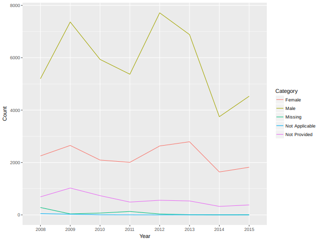
Figure 2: Missingness by Year
2.10 Visualizing Female Proportion Borrowing
The return type of functions in the bigtabulate and biganalytics
packages are base R types that can be used just like you would with
any analysis. This means that we can visualize results using
ggplot2.
In this exercise, you will visualize the female proportion borrowing for urban and rural areas across all years.
2.10.1 Instructions
The matrix prop_female from the previous exercise is available in
your workspace.
- Load the
tidyrandggplot2packages. - Convert
prop_femaleto a data frame usingas.data.frame(). - Add a new column,
Year. Set it to therow.names()ofprop_female_df. - Call
gather()on the columns ofprop_female_dfto convert it into a long format.
## Load the tidyr and ggplot2 packages
Install_And_Load <- function(Required_Packages)
{
        Remaining_Packages <- Required_Packages[!(Required_Packages %in%
                                                  installed.packages()[,"Package"])];

        if(length(Remaining_Packages))
        {
                install.packages(Remaining_Packages, repos='http://cran.rstudio.com/');
        }
        for(package_name in Required_Packages)
        {
                library(package_name,character.only=TRUE,quietly=TRUE);
        }
}

writeLines("\n :: Install new package: tidyr ...")
## Specify the list of required packages to be installed and load
Required_Packages <- c("tidyr", "ggplot2")
## Call the Function
Install_And_Load(Required_Packages);
writeLines("\n :: Library tidyr loaded...")
## -------------------------------------------------------------------

## Convert prop_female to a data frame
prop_female_df <- as.data.frame(prop_female)

## Add a new column Year
prop_female_df$Year <- rownames(prop_female)

## Call gather on prop_female_df
prop_female_long <- gather(prop_female_df, Region, Prop, -Year)

## Create a line plot
## ggplot(prop_female_long, aes(x = Year, y = Prop, group = Region, color = Region)) +
##         geom_line()
:: Install new package: tidyr ...

:: Library tidyr loaded...
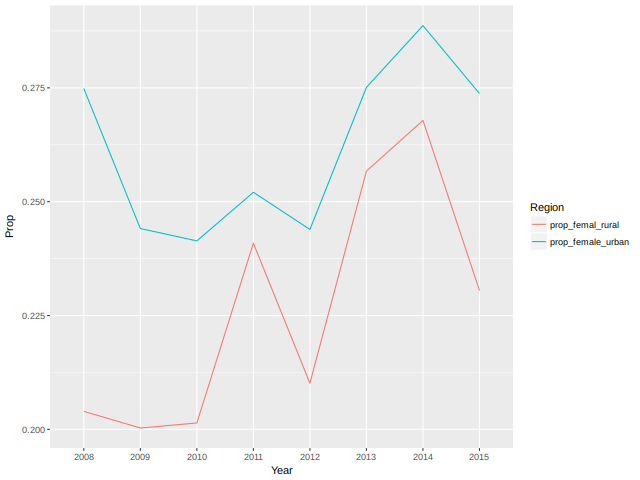
Figure 3: Female proportion borrowing per year
2.11 The Borrower Income Ratio
The borrower income ratio is the ratio of the borrower’s (or borrowers’) annual income to the median family income of the area for the reporting year. This is the ratio used to determine whether borrower’s income qualifies for an income-based housing goal.
In the data set mort, missing values are recoded as 9. In this
exercise, we replaced the 9's in the "borrower_income_ratio" column
with NA, so you can create a table of the borrower income ratios.
2.11.1 Instructions
- Load the
biganalyticsanddplyrpackages. - Call
summary()onmortto check that"borrower_income_ratio"now hasNAs. - Using
bigtable(), create a table of borrower income ratios for each year. - Use
dplyr'smutate()to add a new columnBIR.
## Load biganalytics and dplyr packages
Install_And_Load <- function(Required_Packages)
{
        Remaining_Packages <- Required_Packages[!(Required_Packages %in%
                                                  installed.packages()[,"Package"])];

        if(length(Remaining_Packages))
        {
                install.packages(Remaining_Packages, repos='http://cran.rstudio.com/');
        }
        for(package_name in Required_Packages)
        {
                library(package_name,character.only=TRUE,quietly=TRUE);
        }
}

writeLines("\n :: Install new package: biganalytics ...")
## Specify the list of required packages to be installed and load
Required_Packages <- c("biganalytics", "dplyr")
## Call the Function
Install_And_Load(Required_Packages);
writeLines("\n :: Library biganalytics loaded...")
## -------------------------------------------------------------------

## Call summary on mort
## summary(mort)
mort2 <- deepcopy(mort)
mort2[mort2[, "borrower_income_ratio"] == 9, "borrower_income_ratio"] <- NA
summary(mort2)

bir_df_wide <- bigtable(mort2, c("borrower_income_ratio", "year")) %>%
        ## Turn it into a data.frame
        as.data.frame() %>%
        ## Create a new column called BIR with the corresponding table categories
        mutate(BIR = c(">=0,<=50%", ">50, <=80%", ">80%"))

bir_df_wide
 :: Install new package: biganalytics ...

 :: Library biganalytics loaded...
                               min          max         mean          NAs
enterprise               1.0000000    2.0000000    1.3814571    0.0000000
record_number            0.0000000  999.0000000  499.9080571    0.0000000
msa                      0.0000000    1.0000000    0.8943571    0.0000000
perc_minority            1.0000000    9.0000000    1.9701857    0.0000000
tract_income_ratio       1.0000000    9.0000000    2.3431571    0.0000000
borrower_income_ratio    1.0000000    3.0000000    2.6244912  718.0000000
loan_purpose             1.0000000    9.0000000    3.7670143    0.0000000
federal_guarantee        1.0000000    4.0000000    3.9840857    0.0000000
borrower_race            1.0000000    9.0000000    5.3572429    0.0000000
co_borrower_race         1.0000000    9.0000000    7.0002714    0.0000000
borrower_gender          1.0000000    9.0000000    1.4590714    0.0000000
co_borrower_gender       1.0000000    9.0000000    3.0494857    0.0000000
num_units                1.0000000    4.0000000    1.0398143    0.0000000
affordability            0.0000000    9.0000000    4.2863429    0.0000000
year                  2008.0000000 2015.0000000 2011.2714714    0.0000000
type                     0.0000000    1.0000000    0.5300429    0.0000000
  2008 2009 2010 2011 2012 2013 2014 2015        BIR
1 1205 1473  600  620  745  725  401  380  >=0,<=50%
2 2095 2791 1554 1421 1819 1861 1032 1145 >50, <=80%
3 4844 6707 6609 5934 8338 7559 4255 5169       >80%
2.12 Tidy Big Tables
As a final exercise of using the "tidyverse" packages in combination with the "bigmemory" suite of packages, you will again use the tidyr and ggplot2 packages to plot the Borrower Income ratio over time.
2.12.1 Instructions
- Load the
tidyrandggplot2packages. - Use the
gather()function to gather the counts by year. - Create a line plot with
Yearon the x-axis andCounton the y-axis. Color and group byBIR.
## Load the tidyr and ggplot2 packages
library(tidyr)
library(ggplot2)

## bir_df_wide %>%
##         ## Transform the wide-formatted data.frame into the long format
##         gather(Year, Count, -BIR) %>%
##         ## Use ggplot to create a line plot
##         ggplot(aes(x = Year, y = Count, group = BIR, color = BIR)) +
##         geom_line()
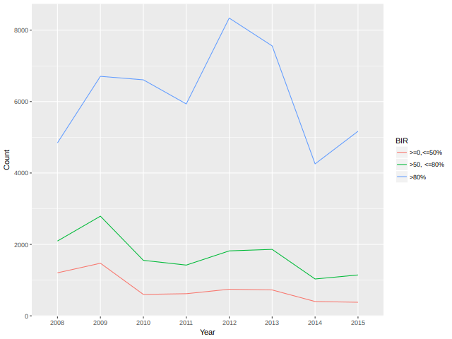
Figure 4: Borrower income ratio plot
You've taken bigmemory to the tidyverse!
2.13 Limitations of bigmemory
video
2.14 Where should you use bigmemory?
The bigmemory package is useful when your data are represented as a
dense, numeric matrix and you can store an entire data set on your
hard drive. It is also compatible with optimized, low-level linear
algebra libraries written in C, like Intel's Math Kernel Library. So,
you can use bigmemory directly in your C and C++ programs for better
performance.
If your data isn't numeric - if you have string variables - or if you
need a greater range of numeric types - like 8-bit integers - then you
might consider trying the ff package. It is similar to bigmemory but
includes a structure similar to a data.frame.
2.14.1 Answer the question
Possible Answers
[ ]You have sparse matrices.[X]You have dense matrices that are at least 10% the size of your total RAM.[ ]You have a large corpus of text data.[ ]You have a matrix that have 50 columns and 50 rows.